
Code
library(tidyverse)
library(emojifont)
library(ggbeeswarm)An analysis of the commercial fish production in the Great Lakes 1867 - 2015. Using beeswarm plots to produce schools of fish. My very first submission for #TidyTuesday!
The #TidyTuesday is a project by the “R for Data Science Online Learning Community”. Each week a well documented dataset provided for the community to explore and visualize. Further information can be found in the github repository.
In week 24 of 2021 the provided dataset is on the commercial fishing production of the Great Lakes (Erie, Superior and Michigan). The dataset description and links to further resources can be found in this weeks data repository.
Thanks to the Great Lakes Fishery Commission for providing the data openly and thanks to the R for Data Science project for cleaning and preparing the dataset.
This is a rather short post, as time ran out before the next release of Tidy Tuesday. I wanted to play around with using icons within plots and the result is an implementation of beeswarm plots that resemble schools of fish. The raw code 1 can be found in my repository. Below is the code to produce the blog version of the plot.
library(tidyverse)
library(emojifont)
library(ggbeeswarm)tuesdata <- tidytuesdayR::tt_load('2021-06-08')#>
#> Downloading file 1 of 2: `stocked.csv`
#> Downloading file 2 of 2: `fishing.csv`glimpse(tuesdata$fishing)#> Rows: 65,706
#> Columns: 7
#> $ year <dbl> 1991, 1991, 1991, 1991, 1991, 1991, 1992, 1992, 1992, 1992…
#> $ lake <chr> "Erie", "Erie", "Erie", "Erie", "Erie", "Erie", "Erie", "E…
#> $ species <chr> "American Eel", "American Eel", "American Eel", "American …
#> $ grand_total <dbl> 1, 1, 1, 1, 1, 1, 0, 0, 0, 0, 0, 0, 0, 0, 0, 0, 0, 0, 0, 0…
#> $ comments <chr> NA, NA, NA, NA, NA, NA, NA, NA, NA, NA, NA, NA, NA, NA, NA…
#> $ region <chr> "Michigan (MI)", "New York (NY)", "Ohio (OH)", "Pennsylvan…
#> $ values <dbl> 0, 0, 0, 0, 0, 1, 0, 0, 0, 0, 0, 0, 0, 0, 0, 0, 0, 0, 0, 0…fishing <- tuesdata$fishing
head(fishing) |> knitr::kable()| year | lake | species | grand_total | comments | region | values |
|---|---|---|---|---|---|---|
| 1991 | Erie | American Eel | 1 | NA | Michigan (MI) | 0 |
| 1991 | Erie | American Eel | 1 | NA | New York (NY) | 0 |
| 1991 | Erie | American Eel | 1 | NA | Ohio (OH) | 0 |
| 1991 | Erie | American Eel | 1 | NA | Pennsylvania (PA) | 0 |
| 1991 | Erie | American Eel | 1 | NA | U.S. Total | 0 |
| 1991 | Erie | American Eel | 1 | NA | Canada (ONT) | 1 |
glimpse(fishing)#> Rows: 65,706
#> Columns: 7
#> $ year <dbl> 1991, 1991, 1991, 1991, 1991, 1991, 1992, 1992, 1992, 1992…
#> $ lake <chr> "Erie", "Erie", "Erie", "Erie", "Erie", "Erie", "Erie", "E…
#> $ species <chr> "American Eel", "American Eel", "American Eel", "American …
#> $ grand_total <dbl> 1, 1, 1, 1, 1, 1, 0, 0, 0, 0, 0, 0, 0, 0, 0, 0, 0, 0, 0, 0…
#> $ comments <chr> NA, NA, NA, NA, NA, NA, NA, NA, NA, NA, NA, NA, NA, NA, NA…
#> $ region <chr> "Michigan (MI)", "New York (NY)", "Ohio (OH)", "Pennsylvan…
#> $ values <dbl> 0, 0, 0, 0, 0, 1, 0, 0, 0, 0, 0, 0, 0, 0, 0, 0, 0, 0, 0, 0…fishing_clean <- fishing |>
mutate(
species = case_when(
str_detect(species, "[Cc]atfish|[Bb]ullhead") ~ "Channel Catfish and Bullheads",
str_detect(species, "[Cc]isco|[Cc]hub") ~ "Cisco and Chubs",
str_detect(species, "[Ww]alleye|(Blue Pike)") ~ "Walleye and Blue Pike",
str_detect(species, "[Rr]ock [Bb]ass|[Cc]rappie") ~ "Rock Bass and Crappie",
str_detect(species, "[Pp]acific [Ss]almon") ~ "Pacific Salmon",
TRUE ~ species
)
) |>
filter(
region %in% c("U.S. Total", "Total Canada (ONT)"),
!is.na(values)
) |>
group_by(species, year) |>
mutate(yearly_total_US_CA = sum(values)) |>
distinct(year, species, yearly_total_US_CA)
fishing_filtered <- fishing_clean |>
group_by(species) |>
summarise(t = sum(yearly_total_US_CA)) |>
filter(t > 500000)
fishing_final <- fishing_clean |>
right_join(fishing_filtered, by = "species")This is a classical line plot showing the commercial production over time for the six most prominent species:
fishing_final |>
  ggplot(
    aes(year, yearly_total_US_CA, color = species)
  ) +
  labs(
    title = "Yearly production of fish in the Great Lakes",
    subtitle = "Combined (US + CA) commercial production of the 6 most prominent species\nof fish in Lakes Erie, Michigan, Superior.",
    x = "Year",
    y = "Commercially produced fish in 1000 pounds",
    caption = "jollydata.blog 2021\nData Source: Great Lakes Fishery Commission."
  ) +
  geom_line() +
  jolly_theme()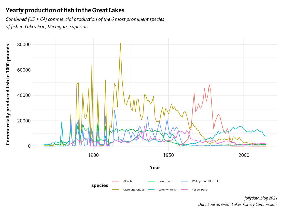
The experimental plot with the beeswarm plots looks like this2:
list.emojifonts()#> [1] "EmojiOne.ttf" "OpenSansEmoji.ttf"load.fontawesome()
load.emojifont("OpenSansEmoji.ttf")
search_emoji('fish')#> [1] "tropical_fish" "fish" "blowfish"
#> [4] "fish_cake" "fishing_pole_and_fish"fishing_final |>
mutate(ktonnes = round(yearly_total_US_CA * 0.4535924 * 0.001)) |>
uncount(ktonnes) |>
ggplot(aes(x=species, y=year, color = species)) +
geom_text(label = emoji("fish"), family="OpenSansEmoji", size=4, alpha = 0.3, position = position_quasirandom(bandwidth = 0.75, varwidth = F)) +
# geom_quasirandom() +
labs(
title = "Commercial Fish Production in the Great Lakes 1867-2015",
subtitle = "Combined (US + CA) commercial production of the 6 most prominent species\nof fish in Lakes Erie, Michigan, Superior.",
x = "Species\n(Each fish-icon represents 1000 tonnes of produced fish.)",
y = "Year",
caption = "\nSource: Great Lakes Fishery Commission | by jollydata.blog 2021 for week 24 of #TidyTuesday"
) +
scale_y_continuous(
breaks = c(1900, 1950, 2000),
minor_breaks = c(1870, 1880, 1890, 1910, 1920, 1930, 1940, 1960, 1970, 1980, 1990, 2010)
) +
scale_color_manual(values = c("#F39F5C", "#EC836D", "#2D7F89", "#E86B72", "#29BCCE", "#56BB83")) +
coord_flip() +
jolly_theme() +
theme(legend.position = "none")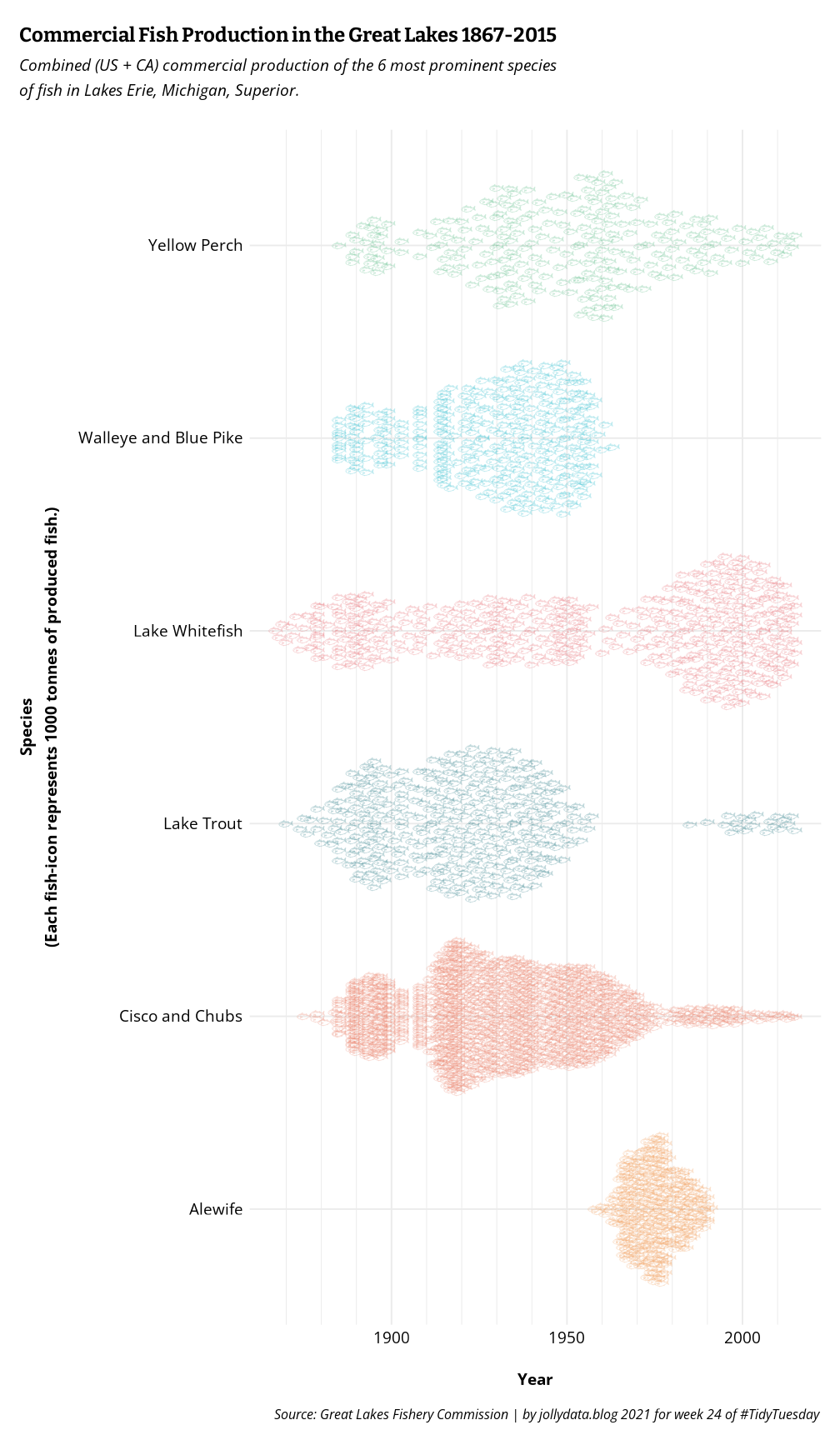
ggsave(last_plot(), filename = "images/2021-24_TT_fishing.pdf",device = "pdf",
                width = 10, height = 20, dpi = 500)
A (rather large) PDF version of the plot can be found here.
The resulting plot gives an overview of the relative yearly productions, similar to a stream plot, without going into too much detail. It shows that there was a relatively short period of an “Alewife burst” coinciding with drastically reduced productions of Cisco, Chubs, Lake Trouts, Walley and Blue Pike.
I enjoyed playing around with the {ggbeeswarm} package and {emojifont} package. Getting the latter one to work in the intended way was rather tedious, but possible in the end.
@online{gebhard2021,
  author = {Gebhard, Christian},
  title = {TidyTuesday 2021 Week 24: {Great} {Lakes} {Commercial}
    {Fishing}},
  date = {2021-06-14},
  url = {https://christiangebhard.com/posts/2021-06-12-tt-fishing/tt-fishing.html},
  langid = {en}
}