When Not in Rome…
…still do as the Romans do. The Roman Empire built many amphitheaters outside of its capital. This post explores 268 of these historic sites and includes a dashboard for interactive exploration.

Introduction
Roman amphitheaters are monumental historic buildings, dating back to the antique times of the Roman Empire. They were mainly used for entertainment, hosting gladiator combats or venationes (animal hunts).
On Amphitheaters
One of the best known amphitheatres is the Colosseum in Rome, also known as the “Flavian Amphitheater”. But over several centuries, the Romans built many more across their Empire. The name describes the architecture: the spectator seats (théatron) are arranged around or on both sides (amphi) of the arena in a circular or oval manner.
Data Source
The dataset comprises historic and geospacial data on 268 theaters1.
Acknowledgements
The data was composed and published by Sebastian Heath from the INSTITUTE FOR THE STUDY OF THE ANCIENT WORLD at NYU. Thanks and credits go to Sebastian Heath, as he published the data under the “Unlicense”, which allowed me to explore and analyse the set for this post.
I stumbled upon this set in the great Data is Plural Newsletter by Jeremy Singer-Vine.
Further Sources
For this post I read articles in several online resources, including
Packages
#> ─ Session info ───────────────────────────────────────────────────────────────
#> setting value
#> version R version 4.2.1 (2022-06-23)
#> os Ubuntu 20.04.5 LTS
#> system x86_64, linux-gnu
#> ui X11
#> language (EN)
#> collate de_DE.UTF-8
#> ctype de_DE.UTF-8
#> tz Europe/Berlin
#> date 2022-09-18
#> pandoc 2.14.2 @ /usr/bin/ (via rmarkdown)
#> quarto 1.1.251 @ /opt/quarto/bin/quarto
#>
#> ─ Packages ───────────────────────────────────────────────────────────────────
#> package * version date (UTC) lib source
#> crosstalk * 1.2.0 2021-11-04 [1] CRAN (R 4.2.0)
#> dplyr * 1.0.9 2022-04-28 [1] CRAN (R 4.2.0)
#> forcats * 0.5.2 2022-08-19 [1] CRAN (R 4.2.1)
#> geomtextpath * 0.1.0.9000 2022-07-07 [1] Github (AllanCameron/geomtextpath@f11e256)
#> ggdist * 3.2.0 2022-07-19 [1] CRAN (R 4.2.1)
#> ggiraph * 0.8.3 2022-08-19 [1] CRAN (R 4.2.1)
#> ggplot2 * 3.3.6 2022-05-03 [1] CRAN (R 4.2.0)
#> ggtext * 0.1.1 2020-12-17 [1] CRAN (R 4.2.1)
#> leaflet * 2.1.1 2022-03-23 [1] CRAN (R 4.2.0)
#> MetBrewer * 0.2.0 2022-03-21 [1] CRAN (R 4.2.0)
#> purrr * 0.3.4 2020-04-17 [3] RSPM (R 4.2.0)
#> reactable * 0.3.0 2022-05-26 [1] CRAN (R 4.2.0)
#> reactablefmtr * 2.1.0 2022-06-05 [1] Github (kcuilla/reactablefmtr@ca67199)
#> readr * 2.1.2 2022-01-30 [1] CRAN (R 4.2.0)
#> sessioninfo * 1.2.2 2021-12-06 [1] CRAN (R 4.2.0)
#> showtext * 0.9-5 2022-02-09 [1] CRAN (R 4.2.0)
#> showtextdb * 3.0 2020-06-04 [1] CRAN (R 4.2.0)
#> stringr * 1.4.1 2022-08-20 [1] CRAN (R 4.2.1)
#> sysfonts * 0.8.8 2022-03-13 [1] CRAN (R 4.2.0)
#> tibble * 3.1.8 2022-07-22 [1] CRAN (R 4.2.1)
#> tidyr * 1.2.0 2022-02-01 [1] CRAN (R 4.2.0)
#> tidyverse * 1.3.2 2022-07-18 [3] RSPM (R 4.2.0)
#>
#> [1] /home/christian/R/x86_64-pc-linux-gnu-library/4.2
#> [2] /usr/local/lib/R/site-library
#> [3] /usr/lib/R/site-library
#> [4] /usr/lib/R/library
#>
#> ──────────────────────────────────────────────────────────────────────────────
Exploratory Data Analysis
Next, let’s read the actual amphitheater data and have a look at it.
Code
# read data and drop columns that won't be used
amphi <- readr::read_csv("https://raw.githubusercontent.com/roman-amphitheaters/roman-amphitheaters/d1b2cb2b401e583cc13837451ed403b42e8fceae/roman-amphitheaters.csv") |>
select(
title, label,
pleiades, buildingtype,
chronogroup, capacity,
modcountry,
arenamajor, arenaminor,
extmajor, extminor,
longitude, latitude, elevation)If you want to see more than the summary, check out the code and output below deck. In there I cover extreme values, distribution of variables and check for spurious correlations.
EDA Summary
There are 268 entries in total and I selected 14 columns of interest.
Missing Data
There are no missing values for the name and location data including coordinates and in which modern country the arena is located now. Other interesting measurements do have missing data unfortunately:
- external theater measurements: 96 missing (35.8%)
- arena measurements: 116 missing (43.3%)
- spectator capacity: 139 missing (51.9%)
Extreme Values
The lowest amphitheater is located in today’s Israel at -134m, the highest at 1170m in Algeria. The one furthest north is located in Newstead (UK), the arena furthest south at Eleutheropolis (Israel).
Below Deck
The following steps were performed to check the validity of the dataset. As this stays below deck, I used base R plots and default colors mostly.
Get an idea of the data
Code
dplyr::glimpse(amphi)#> Rows: 268
#> Columns: 14
#> $ title <chr> "Amphitheater at Dura Europos", "Amphitheater at Arles", …
#> $ label <chr> "Dura", "Arles", "Lyon", "Ludus Magnus", "Colosseum", "Am…
#> $ pleiades <chr> "https://pleiades.stoa.org/places/893989", "https://pleia…
#> $ buildingtype <chr> "amphitheater", "amphitheater", "amphitheater", "practice…
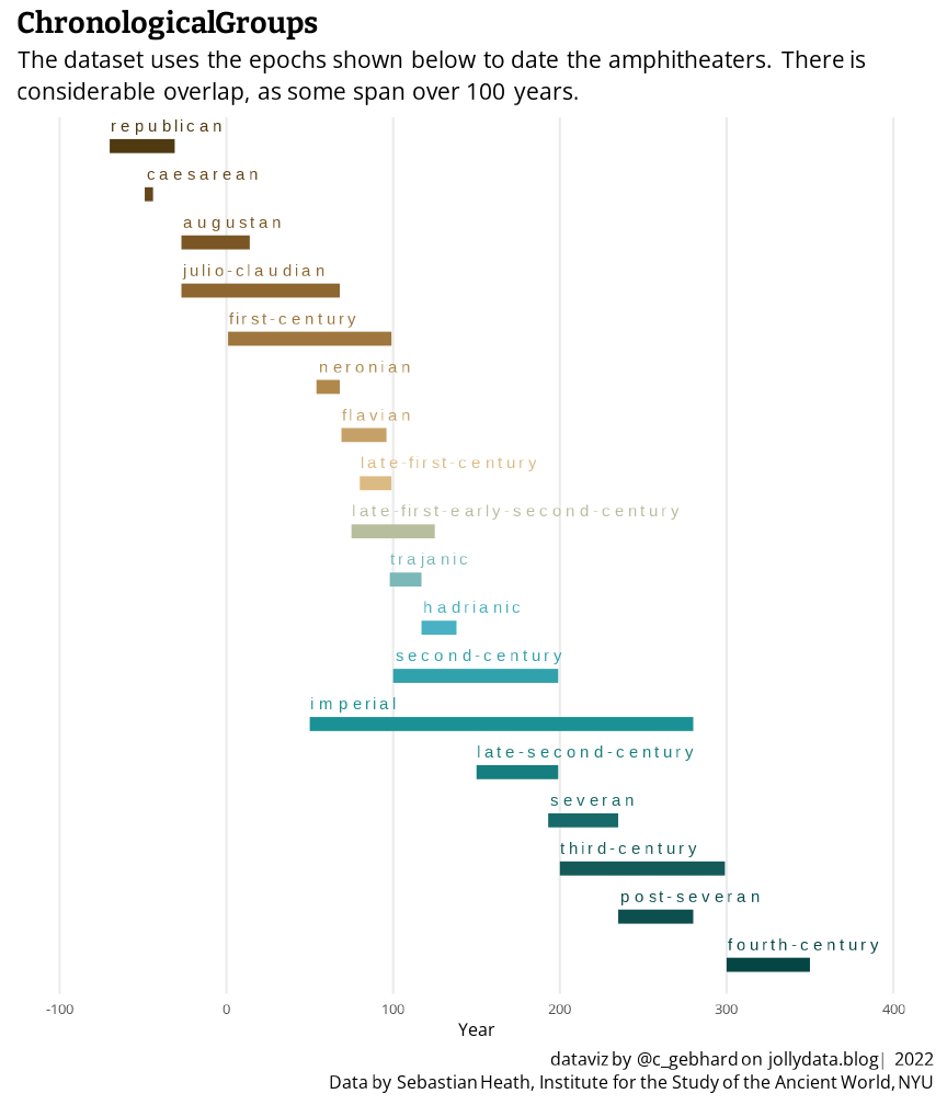
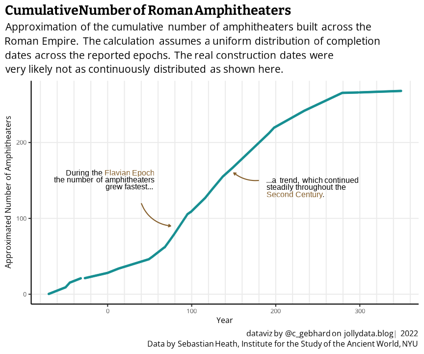
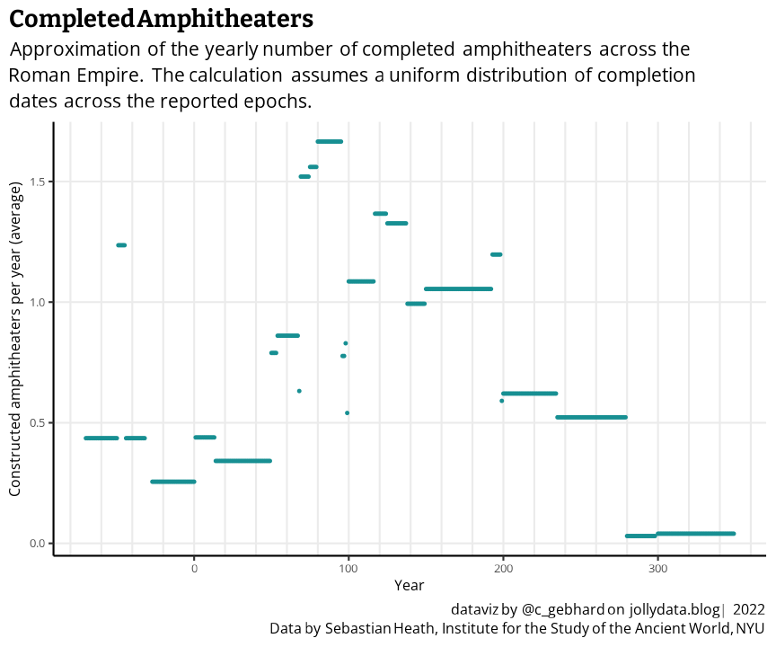
#> $ chronogroup <chr> "severan", "flavian", "second-century", "imperial", "flav…
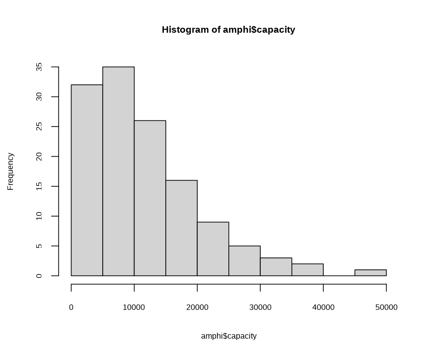
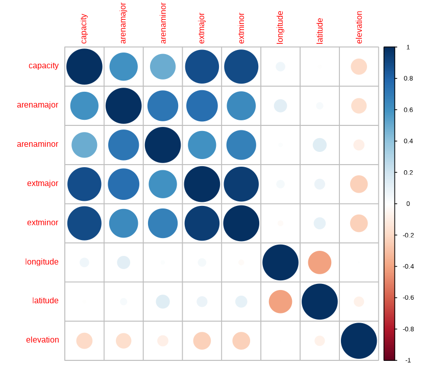
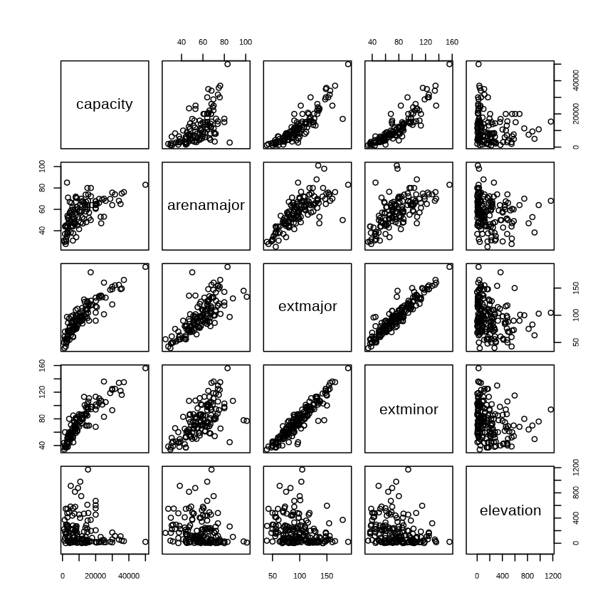
#> $ capacity <dbl> 1000, 23354, 20000, NA, 50000, 7000, 3500, 22000, 15000, …
#> $ modcountry <chr> "Syria", "France", "France", "Italy", "Italy", "Italy", "…
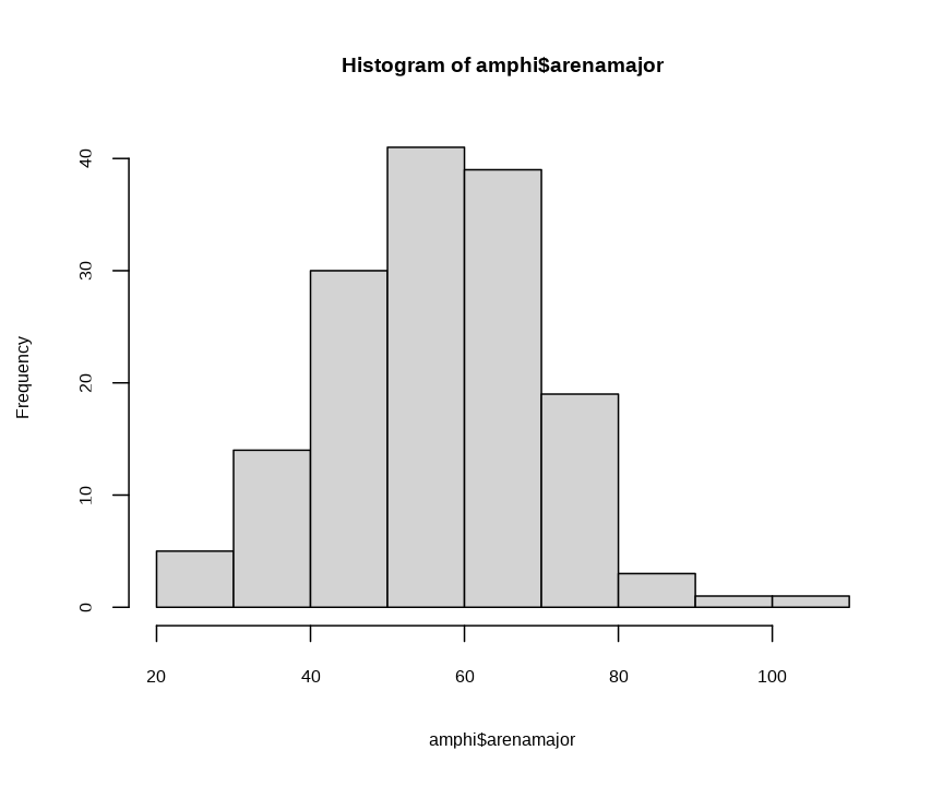
#> $ arenamajor <dbl> 31.0, 47.0, 67.6, NA, 83.0, NA, 47.0, 66.0, 64.0, 37.0, 5…
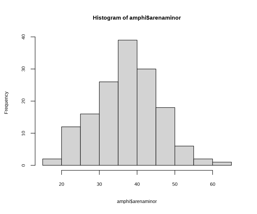
#> $ arenaminor <dbl> 25.0, 32.0, 42.0, NA, 48.0, NA, 38.0, 35.0, 41.0, 23.0, 4…
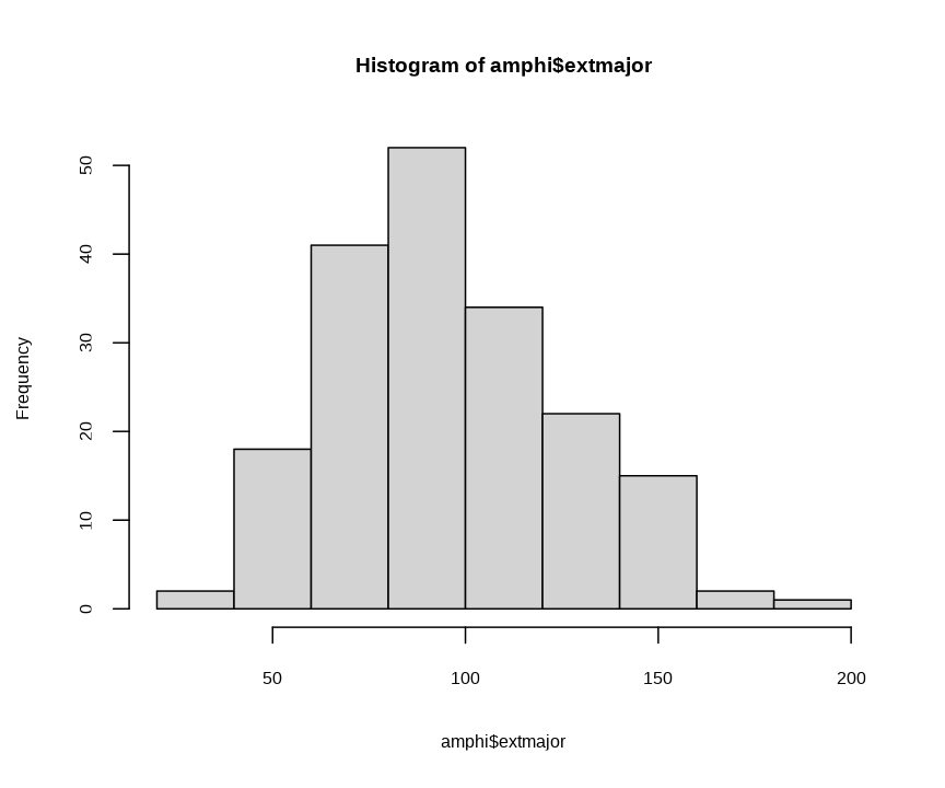
#> $ extmajor <dbl> 50.0, 136.0, 105.0, NA, 189.0, 88.0, 71.0, 135.0, 126.0, …
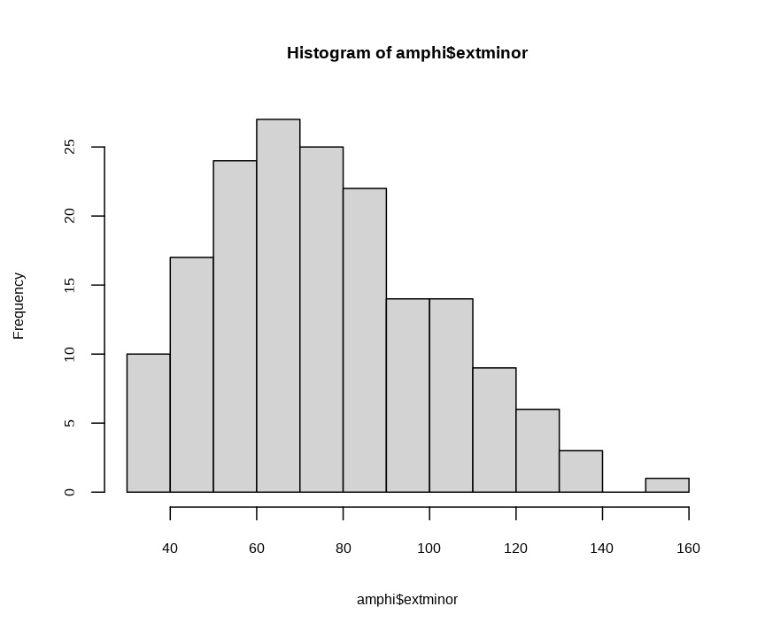
#> $ extminor <dbl> 44.0, 107.0, NA, NA, 156.0, 75.8, 56.0, 104.0, 102.0, 60.…
#> $ longitude <dbl> 40.728926, 4.631111, 4.830556, 12.494913, 12.492269, 12.5…
#> $ latitude <dbl> 34.74985, 43.67778, 45.77056, 41.88995, 41.89017, 41.8877…
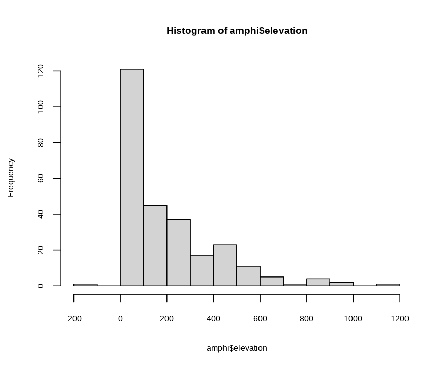
#> $ elevation <dbl> 223, 21, 206, 22, 22, 48, 253, 21, 231, 83, 100, 19, 41, …
Code
head(amphi)#> # A tibble: 6 × 14
#> title label pleia…¹ build…² chron…³ capac…⁴ modco…⁵ arena…⁶ arena…⁷ extma…⁸
#> <chr> <chr> <chr> <chr> <chr> <dbl> <chr> <dbl> <dbl> <dbl>
#> 1 Amphith… Dura https:… amphit… severan 1000 Syria 31 25 50
#> 2 Amphith… Arles https:… amphit… flavian 23354 France 47 32 136
#> 3 Amphith… Lyon https:… amphit… second… 20000 France 67.6 42 105
#> 4 Ludus M… Ludu… https:… practi… imperi… NA Italy NA NA NA
#> 5 Flavian… Colo… https:… amphit… flavian 50000 Italy 83 48 189
#> 6 Amphith… Amph… https:… amphit… severan 7000 Italy NA NA 88
#> # … with 4 more variables: extminor <dbl>, longitude <dbl>, latitude <dbl>,
#> # elevation <dbl>, and abbreviated variable names ¹pleiades, ²buildingtype,
#> # ³chronogroup, ⁴capacity, ⁵modcountry, ⁶arenamajor, ⁷arenaminor, ⁸extmajor
Code
tail(amphi)#> # A tibble: 6 × 14
#> title label pleia…¹ build…² chron…³ capac…⁴ modco…⁵ arena…⁶ arena…⁷ extma…⁸
#> <chr> <chr> <chr> <chr> <chr> <dbl> <chr> <dbl> <dbl> <dbl>
#> 1 Amphith… Tren… https:… amphit… second… NA Italy NA NA NA
#> 2 Amphith… Aven… https:… amphit… second… 13006 Switze… 51 39 99
#> 3 Amphith… Vena… https:… amphit… imperi… 15000 Italy 60 35 110
#> 4 Amphith… Sain… <NA> amphit… first-… 3000 France 54 30 65
#> 5 Amphith… Tole… https:… amphit… imperi… NA Spain NA NA NA
#> 6 Amphith… Kais… https:… amphit… fourth… NA Switze… NA NA 50
#> # … with 4 more variables: extminor <dbl>, longitude <dbl>, latitude <dbl>,
#> # elevation <dbl>, and abbreviated variable names ¹pleiades, ²buildingtype,
#> # ³chronogroup, ⁴capacity, ⁵modcountry, ⁶arenamajor, ⁷arenaminor, ⁸extmajor
Code
summary(amphi)#> title label pleiades buildingtype
#> Length:268 Length:268 Length:268 Length:268
#> Class :character Class :character Class :character Class :character
#> Mode :character Mode :character Mode :character Mode :character
#>
#>
#>
#>
#> chronogroup capacity modcountry arenamajor
#> Length:268 Min. : 1000 Length:268 Min. : 25.00
#> Class :character 1st Qu.: 5150 Class :character 1st Qu.: 47.50
#> Mode :character Median :10000 Mode :character Median : 58.00
#> Mean :12100 Mean : 57.18
#> 3rd Qu.:15550 3rd Qu.: 67.00
#> Max. :50000 Max. :101.00
#> NA's :139 NA's :115
#> arenaminor extmajor extminor longitude
#> Min. :19.00 Min. : 39.60 Min. : 34.00 Min. :-8.493
#> 1st Qu.:32.92 1st Qu.: 75.50 1st Qu.: 58.95 1st Qu.: 5.326
#> Median :38.75 Median : 95.00 Median : 75.00 Median :10.890
#> Mean :38.03 Mean : 97.15 Mean : 76.92 Mean :10.567
#> 3rd Qu.:43.00 3rd Qu.:115.75 3rd Qu.: 94.00 3rd Qu.:14.184
#> Max. :62.00 Max. :189.00 Max. :156.00 Max. :40.729
#> NA's :116 NA's :81 NA's :96
#> latitude elevation
#> Min. :31.61 Min. :-121.00
#> 1st Qu.:38.48 1st Qu.: 34.75
#> Median :42.09 Median : 121.00
#> Mean :42.25 Mean : 196.79
#> 3rd Qu.:45.60 3rd Qu.: 286.25
#> Max. :55.60 Max. :1170.00
#>
Code
dplyr::count(amphi, buildingtype, sort = TRUE)#> # A tibble: 6 × 2
#> buildingtype n
#> <chr> <int>
#> 1 amphitheater 255
#> 2 gallo-roman-amphitheater 6
#> 3 practice-arena 3
#> 4 oval-structure 2
#> 5 arena-in-hippodrome 1
#> 6 arena-in-stadium 1
Code
dplyr::count(amphi, chronogroup, sort = TRUE)#> # A tibble: 18 × 2
#> chronogroup n
#> <chr> <int>
#> 1 imperial 103
#> 2 second-century 54
#> 3 flavian 24
#> 4 first-century 18
#> 5 republican 17
#> 6 julio-claudian 15
#> 7 hadrianic 7
#> 8 severan 6
#> 9 augustan 4
#> 10 caesarean 4
#> 11 late-second-century 3
#> 12 third-century 3
#> 13 fourth-century 2
#> 14 late-first-century 2
#> 15 late-first-early-second-century 2
#> 16 post-severan 2
#> 17 neronian 1
#> 18 trajanic 1
Code
dplyr::count(amphi, modcountry, sort = TRUE)#> # A tibble: 25 × 2
#> modcountry n
#> <chr> <int>
#> 1 Italy 105
#> 2 France 36
#> 3 Tunisia 29
#> 4 Spain 15
#> 5 United Kingdom 15
#> 6 Algeria 8
#> 7 Switzerland 7
#> 8 Turkey 7
#> 9 Austria 6
#> 10 Germany 5
#> # … with 15 more rows
Distribution of numeric variables
Extreme Values
One value caught my eye: the lowest elevation is more than 100m below sea level, which seems odd on first thought. A quick lookup in pleiades and wikipedia however confirms, that the Roman theater of Scythopolis in today’s ‘Beit She’an’ lies below sea level within the Jordan Rift Valley.
The highest located amphitheater is located in today’s Algeria, called ‘Amphitheater at Lambaesis’.
Correlation patterns
Most of the following variable correlations do not make sense in the real world, but this is intended to check for spurious correlations. The strong correlations of external measurements, arena measurements and capacity seem quite plausible.
Code

There is a slight negative correlation between the elevation and the theater measurements, which I cannot explain at this time. To check for visually apparent patterns, we’ll add a scatterplot matrix including the columns that have a Spearman’s \(\rho > 0.1\).
External and Internal Measures of the Amphitheaters
Next up is an analysis of the size of the theaters. Available in the dataset are outer measures and arena size. The amphitheaters usually were of oval shape, so there is a longest possible and a shortest possible axis. Another measure is the capacity of spectators, which will be looked at later.
The buildings and arenas were not always circles. For the calculation of the area we’ll assume, that the shapes are perfect ellipses2.
As preliminary step I derived several variables from the existing columns, such as area and measurements relative to the Colosseum in Rome. The values were stored in amphi.measures. Check out the code below deck, if you like.
Summary
The amphitheater with the largest arena area is located at Utica in Tunisia (the area is given in \(m^2\)). The Colosseum, officially called the “Flavian Amphitheater at Rome”, ranks on place 6 in this category:
#> # A tibble: 6 × 3
#> title arenaarea modcountry
#> <chr> <dbl> <chr>
#> 1 Amphitheater at Utica 3770. Tunisia
#> 2 Amphitheater at Altinum 3644. Italy
#> 3 Amphitheater at Octodurus/Forum Claudii Vallensium 3603. Switzerland
#> 4 Amphitheater at Caesarea 3490. Israel
#> 5 Amphitheater at Lucca 3330. Italy
#> 6 Flavian Amphitheater at Rome 3129. Italy
On the other hand, the Colosseum could – by far – harbor the largest audience:
#> # A tibble: 6 × 3
#> title capacity modcountry
#> <chr> <dbl> <chr>
#> 1 Flavian Amphitheater at Rome 50000 Italy
#> 2 Imperial Amphitheater at Capua 37000 Italy
#> 3 Flavian Amphitheater at Pozzuoli 35700 Italy
#> 4 Amphitheater at Thysdrus 35000 Tunisia
#> 5 Amphitheater at Tours 34000 France
#> 6 Amphitheater at Milan 31649 Italy
To visualize how many people could see an event in the Colosseum, compared to the other venues, we’ll plot the distribution in a raincloud plot. The majority of theaters lie between 5000 to 20000 visitors.
Code
p <- amphi.measures |>
mutate(
is_colosseum = label == "Colosseum",
psize = ifelse(is_colosseum, 3, 0.5)
) |>
ggplot() +
aes(x=1, y = capacity) +
ggdist::stat_halfeye(
fill = "#845d29",
width = .2,
.width = 0,
justification = -2.5,
point_colour = NA,
alpha = 0.85) +
ggdist::stat_pointinterval(
color = "black",
position = position_nudge(x = 0.45),
) +
geom_point_interactive(
aes(tooltip = title, color = is_colosseum, size = psize),
# size = 2,
alpha = .4,
position = position_jitter(
seed = 753, width = .4
)
) +
coord_flip() +
scale_color_met_d("Isfahan1") +
theme_classic() +
labs(
title = "Visitor Capacity of Roman Amphitheaters",
subtitle = "The <span style='color:#178f92; weight: bold;'>Colosseum in Rome</span> is the largest venue with 50k seats.<br>The majority of theaters could fit between 5k and 20k spectators.",
y = "Visitor capacity",
caption = "dataviz by @c_gebhard on jollydata.blog | 2022<br>Data by Sebastian Heath, Institute for the Study of the Ancient World, NYU"
) +
theme(
axis.line.y = element_blank(),
axis.title.y = element_blank(),
axis.text.y = element_blank(),
axis.ticks = element_blank(),
panel.grid.major.x = element_line(color = "#DDDDDD"),
plot.title = element_markdown(family = "Bitter", size = 12, face = "bold"),
plot.subtitle = element_markdown(size = 10),
plot.caption = element_markdown(family = "Bitter", size = 8, lineheight = 1.2),
legend.position = "none"
)
girafe(
ggobj = p,
height_svg = 4
)Distribution of maximum visitor seats at the Amphitheaters across the Roman Empire. The ‘Flavian Amphitheater at Rome’, also known as the ‘Colosseum’, is the largest in terms of spectator seats at ~50000. You can find the points’ names in their tooltips.
Below deck
Code
#> # A tibble: 1 × 6
#> label arenamajor arenaminor extmajor extminor capacity
#> <chr> <dbl> <dbl> <dbl> <dbl> <dbl>
#> 1 Colosseum 83 48 189 156 50000
Code
# calculate different measures
amphi.measures <- amphi |>
mutate(
# measurements
a.frac = arenamajor/arenaminor, # comparison of axes
a.rel.major = arenamajor / 83, # relative to Colosseum
a.rel.minor = arenaminor / 48, # relative to Colosseum
e.frac = extmajor/extminor, # comparison of axes
e.rel.major = extmajor / 189, # relative to Colosseum
e.rel.minor = extminor / 156, # relative to Colosseum
# capacity
cap.rel = capacity / 50000,
# area
extarea = 0.5*extmajor * 0.5*extminor * pi,
arenaarea = 0.5 * arenamajor * 0.5 * arenaminor * pi,
)The Roman Amphitheaters across the Centruries
The dataset ranges from the republican era (starting around the year 70 BC) until the mid 4th century AD. The construction dates given in the dataset are not exactly specified on a year-level. This is understandable, as there might not be exact dates written on records or the cornerstones. Dating might rely on a combination architectural characteristics, historic texts and records. The diagram below displays the time scales of the epochs used in this dataset.
Code
# read the dataset
chrono <- readr::read_csv("https://raw.githubusercontent.com/roman-amphitheaters/roman-amphitheaters/d1b2cb2b401e583cc13837451ed403b42e8fceae/chronogrps.csv")
# rearrange for plotting
chrono_long <- chrono |>
pivot_longer(cols = c(startdate, enddate), names_to = "date_type", values_to = "date")
ggplot(chrono_long) +
aes(
x = reorder(id, date, decreasing = TRUE),
y = date
) +
geom_textline(
aes(
label = id,
color = reorder(id, date, decreasing = TRUE)
),
vjust = -0.4,
hjust = 0,
linewidth = 3,
size = 4
) +
scale_color_manual(values = met.brewer("Isfahan1", 18, type = "continuous", direction = -1)) +
scale_y_continuous(limits = c(-100, 400)) +
coord_flip() +
labs(
y = "Year",
title = "Chronological Groups",
subtitle = "The dataset uses the epochs shown below to date the amphitheaters. There is<br>considerable overlap, as some span over 100 years.",
caption = "dataviz by @c_gebhard on jollydata.blog | 2022<br>Data by Sebastian Heath, Institute for the Study of the Ancient World, NYU"
) +
theme_classic() +
theme(
axis.line = element_blank(),
axis.text.y = element_blank(),
axis.title.y = element_blank(),
axis.ticks = element_blank(),
legend.position = "none",
text = element_text(family = "Open Sans", size = 12),
panel.grid.major.x = element_line(),
plot.title = element_markdown(family = "Bitter", size = 20, face = "bold"),
plot.subtitle = element_markdown(size = 16),
plot.caption = element_markdown(size = 12)
)
Which was the most prolific epoch, defined as ‘most amphitheaters constructed’? This is difficult to say, as the chronological groups are relatively unspecific. There are two approaches, both are ‘history-agnostic’. By that I mean, that I do not have any historic expert knowledge, nor did I do any research first. Both approaches are based on the data itself.
Mean buildings per epoch
A possible first approach is a mean construction count per year for each chronological group.
Top 6 chronological groups
Code
#> # A tibble: 6 × 4
#> chronogroup n_amphi duration amphi_per_year
#> <chr> <int> <dbl> <dbl>
#> 1 flavian 24 27 0.889
#> 2 caesarean 4 5 0.8
#> 3 second-century 54 99 0.545
#> 4 imperial 103 230 0.448
#> 5 republican 17 39 0.436
#> 6 hadrianic 7 21 0.333
Below deck
Code
# calculate epoch duration
chrono.duration <- chrono |>
mutate(
duration = enddate - startdate
)
# count constructions per chronogroup and join the duration
amphi.duration <- amphi |>
count(chronogroup) |>
left_join(chrono.duration, by = c("chronogroup" = "id")) |>
rename(n_amphi = n)
# calculate constructions per epoch
amphi.construct <- amphi.duration |>
mutate(amphi_per_year = n_amphi / duration) |>
arrange(desc(amphi_per_year))The most ‘prolific’ epoch in this view would be the ‘flavian’ epoch with 0.889 amphitheaters built per year (see amphi_per_year in the table above).3 The problem with this approach is the overlapping of several groups. Theaters built in the flavian age would in reality also count as being built e.g. during the ‘late first century’ or partially in the ‘late first early second century’. The dataset however cannot represent this, as each amphitheater is only assigned one of the chronological groups.
Yearly approximation
The second approach tackles the limitation of the previous attempt by summing the average constructions per year of all epochs on a yearly scale. The key assumption here is a uniform distribution4 of the constructions within each epoch. In other words, we assume, that the finalization of amphitheaters is evenly spread across all years of an epoch. The necessary data preparation can be found below deck.
Cumulative
Code
ggplot(amphi.years.cumul) +
aes(x = year, y = y_cumsum) +
geom_point(
size = 0.5,
color = "#178f92"
) +
labs(
x = "Year",
y = "Approximated Number of Amphitheaters",
title = "Cumulative Number of Roman Amphitheaters",
subtitle = "Approximation of the cumulative number of amphitheaters built across the<br>Roman Empire. The calculation assumes a uniform distribution of completion<br>dates across the reported epochs. The real construction dates were<br>very likely not as continuously distributed as shown here.",
caption = "dataviz by @c_gebhard on jollydata.blog | 2022<br>Data by Sebastian Heath, Institute for the Study of the Ancient World, NYU"
) +
scale_x_continuous(
minor_breaks = seq(-100, 400, 20)
) +
theme_classic() +
theme(
panel.grid.minor.x = element_line(),
panel.grid.major.x = element_line(),
panel.grid.major.y = element_line(),
text = element_text(family = "Open Sans", size = 12),
plot.title = element_markdown(family = "Bitter", size = 20, face = "bold"),
plot.subtitle = element_markdown(size = 16),
plot.caption = element_markdown(size = 12),
plot.title.position = "plot"
) +
annotate(
geom = "richtext",
label = "<span style='font-family: Open Sans; font-size: 12pt;'>During the <span style='color: #845d29;'><b>Flavian Epoch</b></span><br> the number of amphitheaters<br>grew fastest...</span>",
x = 60,
y = 150,
hjust = 1,
lineheight = 0.6,
fill = NA,
label.color = NA
) +
annotate(
geom = "curve", x = 180, y = 150, xend = 150, yend = 160,
curvature = -.2, arrow = arrow(length = unit(1, "mm")),
color = "#845d29"
) +
annotate(
geom = "richtext",
label = "<span style='font-family: Open Sans; font-size: 12pt;'>...a trend, which continued<br>steadily throughout the<br><span style='color: #845d29;'><b>Second Century</b></span>.</span>",
x = 185,
y = 140,
hjust = 0,
lineheight = 0.6,
fill = NA,
label.color = NA
) +
annotate(
geom = "curve", x = 40, y = 120, xend = 75, yend = 90,
curvature = .3, arrow = arrow(length = unit(1, "mm")),
color = "#845d29"
)
Yearly Average
Code
ggplot(amphi.years.cumul) +
aes(x = year, y = y_cumul) +
geom_point(
size = 0.5,
color = "#178f92"
) +
labs(
x = "Year",
y = "Constructed amphitheaters per year (average)",
title = "Completed Amphitheaters",
subtitle = "Approximation of the yearly number of completed amphitheaters across the<br>Roman Empire. The calculation assumes a uniform distribution of completion<br> dates across the reported epochs.",
caption = "dataviz by @c_gebhard on jollydata.blog | 2022<br>Data by Sebastian Heath, Institute for the Study of the Ancient World, NYU"
) +
scale_x_continuous(
minor_breaks = seq(-100, 400, 20)
) +
theme_classic() +
theme(
panel.grid.minor.x = element_line(),
panel.grid.major.x = element_line(),
panel.grid.major.y = element_line(),
text = element_text(family = "Open Sans", size = 12),
plot.title = element_markdown(family = "Bitter", size = 20, face = "bold"),
plot.subtitle = element_markdown(size = 16),
plot.caption = element_markdown(size = 12),
plot.title.position = "plot"
)
Below deck
Code
## add rows for all years between start and end date of an epoch:
amphi.years <- amphi.construct |>
# create dummy rows for each year of an epoch (number equals duration)
uncount(duration) |>
# group by epoch
group_by(chronogroup) |>
# add row number (within each group) to epoch's start year to create a continuous year sequence for each epoch
# ranging from the start date to the end date
mutate(
year = startdate + 1:n() - 1
) |>
ungroup()
## obtain yearly sums
amphi.years.cumul <- amphi.years |>
# group by year
group_by(year) |>
# summarise all fractional yearly amphitheaters of all epochs in a given year
summarise(y_cumul = sum(amphi_per_year)) |>
# calculate the cumulative sum over the years
arrange(year) |>
mutate(
y_cumsum = cumsum(y_cumul)
)Code
# check if all yearly fractional amphitheaters over the complete time span
# matches the number of amphitheaters in the dataset
sum(amphi.years.cumul$y_cumul)#> [1] 268
Where are the Amphitheaters located now?
In the final section of the exploratory analysis, we’ll see where the Romans built the most theaters.
#> # A tibble: 10 × 2
#> modcountry n
#> <chr> <int>
#> 1 Italy 105
#> 2 France 36
#> 3 Tunisia 29
#> 4 Spain 15
#> 5 United Kingdom 15
#> 6 Algeria 8
#> 7 Switzerland 7
#> 8 Turkey 7
#> 9 Austria 6
#> 10 Germany 5
By far, the Romans built most theaters on their “home turf” (105 in total), which is now Italian territory. France follows on the list with 36, Tunisia with 29. Spain and the UK each have 15 amphitheaters on record.
All in all the Romans left their cultural mark (in terms of amphitheaters) in 25 countries.
Dashboard: Explore the Data by Yourself
This section is intended for you, the reader, to explore the data by yourself.5 The code for the interactive dashboard can be found below deck.
How to use
In the top left, you can filter for one or more epochs or specify a range of spectators to filter the amphitheaters in the map and the table below. You can also search the table via the searchbox on the top right of the table. If you select one or more in the table, they will be highlighted on the map. On the other hand, if you explore the map and want want to see more information on the selected theater, just click on the button in the popup to jump to the entry in the table. (To get back to the full table, simply empty the search box of the table.)
Below Deck
Code
amphi.react <- amphi |>
mutate(
title_html = paste0(
"<b>", .data$title, "</b><br><br>",
'<button onclick="Reactable.setSearch(\'amphi-table\',\'',
.data$title,
'\')">',
"Show in table",
'</button>'
),
cap.fixed = ifelse(is.na(capacity), 0, capacity)
) |>
relocate(title, chronogroup, modcountry) |>
arrange(desc(capacity))
# Wrap data frame in SharedData
crosstalk_data <- SharedData$new(amphi.react)
### crosstalk epoch filter, a textbox that allows multiple selections of epochs
epoch_filter <- filter_select(
id = "epoch",
label = "EPOCH",
sharedData = crosstalk_data,
group = ~ chronogroup
)
### crosstalk YEAR filter, a slider elemtn to select year-ranges
cap_filter <- filter_slider(
id = "capacity",
label = "CAPACITY",
sharedData = crosstalk_data,
column = ~ cap.fixed,
ticks = TRUE,
dragRange = FALSE,
step = 1000,
sep = "",
width = "90%"
)
### Build the table
amphi.table <- reactable(
crosstalk_data,
theme = default(),
showSortIcon = TRUE,
searchable = TRUE,
selection = "multiple",
onClick = "select",
elementId = "amphi-table",
columns = list(
title_html = colDef(show = FALSE),
label = colDef(show = FALSE),
buildingtype = colDef(show = FALSE),
cap.fixed = colDef(show = FALSE),
latitude = colDef(show = FALSE),
longitude = colDef(show = FALSE),
pleiades = colDef(show = FALSE),
arenaminor = colDef(show = FALSE),
extminor = colDef(show = FALSE),
title = colDef(
name = "Name"
),
chronogroup = colDef(
name = "Epoch"
),
modcountry = colDef(
name = "Modern Country"
),
capacity = colDef(
name = "Spectator Capacity",
cell = data_bars(
data = amphi.react,
fill_color = met.brewer("Isfahan1", 5),
background = '#F1F1F1',
min_value = 0,
max_value = 50000,
text_position = 'inside-end',
force_outside = c(0,20001),
number_fmt = scales::comma
)
),
arenamajor = colDef(
name = "Arena major axis (m)",
maxWidth = 75,
cell = data_bars(
data = amphi.react,
fill_color = met.brewer("Isfahan1", 5),
background = '#F1F1F1',
min_value = 0,
max_value = 101,
text_position = 'inside-end',
force_outside = c(0,30),
number_fmt = scales::comma
)
),
extmajor = colDef(
name = "External major axis (m)",
maxWidth = 75,
cell = data_bars(
data = amphi.react,
fill_color = met.brewer("Isfahan1", 5),
background = '#F1F1F1',
min_value = 0,
max_value = 189,
text_position = 'inside-end',
force_outside = c(0,70),
number_fmt = scales::comma
)
),
elevation = colDef(
name = "Elevation (m)",
maxWidth = 75
)
)
) |>
add_source(
source = 'Data by Sebastian Heath, Institute for the Study of the Ancient World, NYU',
font_style = 'italic',
font_size = 12
)
### display and arrange the widgets
htmltools::div(
# style = "justify-content: center;",
bscols(
widths = c(4, 8),
list(
epoch_filter,
cap_filter
),
leaflet(crosstalk_data) %>% addTiles() %>% addMarkers(popup = amphi.react$title_html)
)
)
htmltools::div(
amphi.table
)Data by Sebastian Heath, Institute for the Study of the Ancient World, NYU
Final Thoughts and Comments
After a long time I got back, to where I started the blog: grab an open dataset and do some exploration of the data. On the way I got more proficient in using crosstalk to link a map widget with an interactive table. There is still some room for improvement (e.g. I couldn’t figure out how to select several locations on the map and filter for those in the table). If you enjoyed reading the post or even learned something as well, or know how to improve the article, feel free to leave a comment below.
Footnotes
that is at the time of writing. The dataset might have been updated in the meantime↩︎
The area A is thus: \(A=a\cdot b\cdot\pi\), where \(a\) is the half major axis, \(b\) is the half minor axis↩︎
The Colosseum, aka the ‘Flavian Amphitheater’ was built between 72 and 80 AD and falls into this epoch.↩︎
https://en.wikipedia.org/wiki/Discrete_uniform_distribution↩︎
Also: I wanted to learn how to build interactive ‘dashboards’ that run client-side without the need to have a shiny server in the background.↩︎
Reuse
Citation
@online{gebhard2022,
author = {Gebhard, Christian},
title = {When {Not} in {Rome...}},
date = {2022-07-08},
url = {https://christiangebhard.com/posts/2022-06-12-when-not-in-rome/when-not-in-rome.html},
langid = {en}
}


